Analytic Geometry

Analytic geometry is the study of geometry in 2D and 3D space using coordinate systems and algebraic methods. It provides the geometric framework in which linear algebra operates, giving visual and spatial meaning to vectors, matrices, and linear transformations.

In this section we will cover the more elementary aspects of analytic geometry in relation to the basic components of linear algebra (vectors and matrices). In particular, it covers the geometric interpretation of vectors in coordinate systems, equations for planes in three-dimensional space, and the linear transformations that operate on these geometric objects. A more detailed description of linear algebra in 2D and 3D space can be found in the next chapter entitled Geometry.

Vectors in Coordinate Systems

While Vectors covers the algebraic properties of vectors, here we focus on their geometric interpretation in coordinate systems — vectors as directed distances between points.

Vectors as Directed Distances

A vector in $\mathbb{R}^2$ represents a directed distance: starting from any point, move $a_1$ steps horizontally and $a_2$ steps vertically to reach the endpoint. The vector $\mathbf{a}$ can be drawn anywhere in the plane and records only these displacements — not the starting point: $\mathbf{a} = \begin{pmatrix} a_1 \\ a_2 \end{pmatrix}$

In $\mathbb{R}^3$, starting from any point, move $a_1$ steps horizontally, $a_2$ steps vertically, and $a_3$ steps in depth to reach the endpoint. Here too, the vector can be drawn anywhere in space: $\mathbf{a} = \begin{pmatrix} a_1 \\ a_2 \\ a_3 \end{pmatrix}$

Connecting Vectors

Given two points $A = (x_A, y_A)$ and $B = (x_B, y_B)$, the connecting vector $\vec{AB}$ is the displacement needed to travel from point $A$ to $B$: $\vec{AB} = \begin{pmatrix} x_B - x_A \\ y_B - y_A \end{pmatrix}$

In $\mathbb{R}^3$, for points $A = (x_A, y_A, z_A)$ and $B = (x_B, y_B, z_B)$: $\vec{AB} = \begin{pmatrix} x_B - x_A \\ y_B - y_A \\ z_B - z_A \end{pmatrix}$

2D Example: For $A = (1, 2)$ and $B = (3, 5)$, the connecting vector is $\vec{AB} = \begin{pmatrix} 2 \\ 3 \end{pmatrix}$ — move 2 steps horizontally and 3 steps vertically.

3D Example: For $A = (1, 2, 3)$ and $B = (4, 0, 1)$, the connecting vector is $\vec{AB} = \begin{pmatrix} 3 \\ -2 \\ -2 \end{pmatrix}$ — move 3 steps horizontally, 2 steps down, and 2 steps back in depth.

The connecting vector depends on both $A$ and $B$ — choosing a different starting point gives a different displacement. What defines the vector is the relative displacement between the two points, not their absolute positions: shifting both $A$ and $B$ by the same amount leaves $\vec{AB}$ unchanged.

Position Vectors

A position vector (or location vector) is the special case where the starting point is the origin $O$. The position vector of a point $A = (x_A, y_A)$ is: $\vec{OA} = \begin{pmatrix} x_A \\ y_A \end{pmatrix}$

The position vector has the same coordinates as the point itself — it describes how to travel from the origin to the given location.

In $\mathbb{R}^3$, the position vector of $A = (x_A, y_A, z_A)$ is: $\vec{OA} = \begin{pmatrix} x_A \\ y_A \\ z_A \end{pmatrix}$

Any connecting vector can be expressed as the difference of two position vectors: $\vec{AB} = \vec{OB} - \vec{OA}$. We need to point out a subtle distinction — $A$ and $B$ are points (locations in space), while $\vec{OA}$ and $\vec{OB}$ are vectors (displacements from the origin). The statement above is referring to vector subtraction, not point subtraction: it is the vectors that carry the arithmetic, not the points themselves.

Geometric Interpretation of Operations

Vector operations have direct geometric meaning in coordinate systems:

Negation: $-\mathbf{a}$ reverses the direction of $\mathbf{a}$. If $\mathbf{a} = \vec{AB}$ then $-\mathbf{a} = \vec{BA}$
Scalar multiplication: $\lambda \mathbf{a}$ stretches $\mathbf{a}$ by factor $\lvert \lambda \rvert$ in the same direction (if $\lambda > 0$) or the opposite direction (if $\lambda < 0$)
Addition: To compute $\mathbf{a} + \mathbf{b}$ geometrically, place the start of $\mathbf{b}$ at the end of $\mathbf{a}$; the sum is the vector from the start of $\mathbf{a}$ to the end of $\mathbf{b}$
Subtraction: $\mathbf{a} - \mathbf{b}$ is equivalent to adding the negation: $\mathbf{a} + (-\mathbf{b})$. Geometrically, reverse $\mathbf{b}$ and then add it to $\mathbf{a}$. This is how connecting vectors are computed: $\vec{AB} = \vec{OB} - \vec{OA}$ subtracts two position vectors to produce a displacement

For the algebraic rules behind these operations, see Vector Operations.

Planes in Space

A plane in three-dimensional space is uniquely determined by three non-collinear points. Plane equations come in two forms: the parameterized form using direction vectors, and the parameter-free form using a normal vector.

Parameterized Form

Definition

Given three non-collinear points $A$, $B$, and $C$ in $\mathbb{R}^3$, any point $\mathbf{x}$ on the plane through them can be written as: $\mathbf{x} = \mathbf{a} + \lambda \mathbf{b} + \mu \mathbf{c}$ where:

The position vector of $A$ is $\mathbf{a} = \vec{OA}$ where $O$ is the origin point $(0, 0, 0)$
The connecting vector from $A$ to $B$ is $\mathbf{b} = \vec{AB}$
The connecting vector from $A$ to $C$ is $\mathbf{c} = \vec{AC}$
The free parameters are $\lambda, \mu \in \mathbb{R}$

The vectors $\mathbf{b}$ and $\mathbf{c}$ span the plane — every point on the plane can be reached from $A$ by some linear combination of these two direction vectors.

Derivation

Vectors in a plane

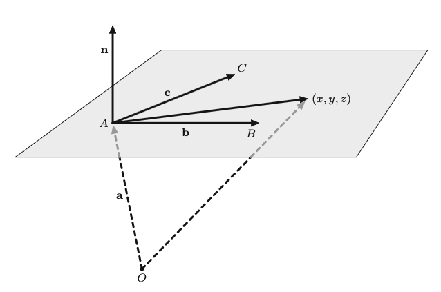
In order to derive the parameterized form equation, let's look at the diagram above. First, we have the three points $A$, $B$ and $C$ which lie in the plane. And we want to define the vector from $O$ to any arbitrary point $P = (x, y, z)$ in the same plane as $A$. Using the origin $O = (0, 0, 0)$ we can write the equation $\vec{OP} = \vec{OA} + \vec{AP}$ that is we go from the origin to point A and from A we travel to the arbitrary point P on the same plane. Since $\vec{AB}$ and $\vec{AC}$ also lie on the same plane, $\vec{AP} = \lambda \vec{AB} + \mu \vec{AC}$. This directly leads to the equation defined in the previous section.

Example

For the plane through $A = (1, 2, 3)$, $B = (0, 1, 2)$, and $C = (-1, 2, 1)$:

\[\begin{aligned} \mathbf{a} &= \begin{pmatrix} 1 \\ 2 \\ 3 \end{pmatrix}, \quad \mathbf{b} = \vec{AB} = \begin{pmatrix} -1 \\ -1 \\ -1 \end{pmatrix}, \quad \mathbf{c} = \vec{AC} = \begin{pmatrix} -2 \\ 0 \\ -2 \end{pmatrix} \end{aligned}\]

The parameterized equation is: $\begin{pmatrix} x \\ y \\ z \end{pmatrix} = \begin{pmatrix} 1 \\ 2 \\ 3 \end{pmatrix} + \lambda \begin{pmatrix} -1 \\ -1 \\ -1 \end{pmatrix} + \mu \begin{pmatrix} -2 \\ 0 \\ -2 \end{pmatrix}$

Setting $\lambda = 0, \mu = 0$ gives the point $(1, 2, 3) = A$ itself.

Parameter-Free Form

Normal Vectors

A normal vector $\mathbf{n}$ to a plane is a vector that is perpendicular to every vector lying in the plane.

The normal vector can be found by solving a derived system of linear equations as shown in the example below. Or, more directly, by using the cross product described in the next section.

Example Let's return to the example used in the Parameterized Form section above. See the diagram in the Derivation section. We have two vectors in the plane from the example:

\[\begin{aligned} \mathbf{b} = \vec{AB} = \begin{pmatrix} -1 \\ -1 \\ -1 \end{pmatrix}, \quad \mathbf{c} = \vec{AC} = \begin{pmatrix} -2 \\ 0 \\ -2 \end{pmatrix} \end{aligned}\]

The diagram also indicates the normal vector $\mathbf{n} = \begin{pmatrix} n_1 \\ n_2 \\ n_3 \end{pmatrix}$.

Recall that two vectors are perpendicular if and only if their dot product is zero ($\mathbf{a} \cdot \mathbf{b} = 0$) which holds in both $\mathbb{R}^2$ and $\mathbb{R}^3$. Hence, for the plane spanned by $\mathbf{b}$ and $\mathbf{c}$, the normal vector must satisfy both $\mathbf{n} \cdot \mathbf{b} = 0$ and $\mathbf{n} \cdot \mathbf{c} = 0$. Thus:

\[\begin{aligned} 0 = \mathbf{n} \cdot \mathbf{b} = \begin{pmatrix} n_1 \\ n_2 \\ n_3 \end{pmatrix} \cdot \begin{pmatrix} -1 \\ -1 \\ -1 \end{pmatrix} = -n_1-n_2-n_3 \\ 0 = \mathbf{n} \cdot \mathbf{c} = \begin{pmatrix} n_1 \\ n_2 \\ n_3 \end{pmatrix} \cdot \begin{pmatrix} -2 \\ 0 \\ -2 \end{pmatrix} = -2n_1-2n_3 \end{aligned}\]

This gives us a linear system of two equations in three unknowns and can be solved using the techniques described in the System of Equations.

Cross Product

The cross product (vector product) of two 3D vectors $\mathbf{b}$ and $\mathbf{c}$ gives a vector perpendicular to both: $\mathbf{b} \times \mathbf{c} = \begin{pmatrix} b_2c_3 - b_3c_2 \\ b_3c_1 - b_1c_3 \\ b_1c_2 - b_2c_1 \end{pmatrix}$

The cross product provides the normal vector directly without solving a system of equations.

If the cross product yields the zero vector, the three points are collinear (lie on a line) and no unique plane exists.

Example (continued): Using the vectors from above:

\[\mathbf{n} = \mathbf{b} \times \mathbf{c} = \begin{pmatrix} -1 \\ -1 \\ -1 \end{pmatrix} \times \begin{pmatrix} -2 \\ 0 \\ -2 \end{pmatrix} = \begin{pmatrix} (-1)(-2) - (-1)(0) \\ (-1)(-2) - (-1)(-2) \\ (-1)(0) - (-1)(-2) \end{pmatrix} = \begin{pmatrix} 2 \\ 0 \\ -2 \end{pmatrix}\]

If we calculate the dot product of $\mathbf{n}$ and $\mathbf{b}$ and $\mathbf{n}$ and $\mathbf{c}$ the result is 0 as expected and required for n to be the normal vector.

Parameter-Free Plane Equation

Given three non-collinear points $A = (a_1, a_2, a_3)$, $B = (b_1, b_2, b_3)$, and $C = (c_1, c_2, c_3)$, the parameter-free equation of the plane through them is computed as follows:

Step 1 Determine the position vector $\mathbf{a}$ and the direction vectors $\mathbf{b} = \vec{AB}$ and $\mathbf{c} = \vec{AC}$:$\mathbf{a} = \begin{pmatrix} a_1 \\ a_2 \\ a_3 \end{pmatrix}, \qquad \mathbf{b} = \begin{pmatrix} b_1 - a_1 \\ b_2 - a_2 \\ b_3 - a_3 \end{pmatrix}, \qquad \mathbf{c} = \begin{pmatrix} c_1 - a_1 \\ c_2 - a_2 \\ c_3 - a_3 \end{pmatrix}$

Step 2 Calculate the normal vector using the cross product:$\mathbf{n} = \mathbf{b} \times \mathbf{c} = \begin{pmatrix} b_2 c_3 - b_3 c_2 \\ b_3 c_1 - b_1 c_3 \\ b_1 c_2 - b_2 c_1 \end{pmatrix}$

Step 3 For a plane point $(x, y, z)$, set up the dot product condition — since $\mathbf{n}$ is perpendicular to every vector in the plane, in particular to the connecting vector from $A$ to any plane point:$\mathbf{n} \cdot \begin{pmatrix} x - a_1 \\ y - a_2 \\ z - a_3 \end{pmatrix} = 0$

Step 4 Expand the dot product and simplify until the equation takes the form $ax + by + cz = d$. This is the parameter-free equation of the plane.

The equation is called parameter-free because it contains no free parameters $\lambda$ or $\mu$, only the coordinates $(x, y, z)$ of an arbitrary point on the plane. As noted earlier, we know the three points lie on a plane and not a straight line, when the vector product $\mathbf{b} \times \mathbf{c}$ is not the zero vector.

Example (continued):

Going back to our example, with points $A = (1, 2, 3)$, $B = (0, 1, 2)$, and $C = (-1, 2, 1)$:

Step 1 Determine the three vectors: $\begin{aligned} \mathbf{a} &= \begin{pmatrix} 1 \\ 2 \\ 3 \end{pmatrix}, \quad \mathbf{b} = \vec{AB} = \begin{pmatrix} -1 \\ -1 \\ -1 \end{pmatrix}, \quad \mathbf{c} = \vec{AC} = \begin{pmatrix} -2 \\ 0 \\ -2 \end{pmatrix} \end{aligned}$

Step 2 Determine the normal vector:

Step 3 For a plane point $(x, y, z)$ set up dot product condition:

\[\begin{pmatrix} 2 \\ 0 \\ -2 \end{pmatrix} \cdot \begin{pmatrix} x - 1 \\ y - 2 \\ z - 3 \end{pmatrix} = 2(x - 1) + 0(y - 2) - 2(z - 3) = 2x - 2z + 4 = 0\]

Step 4 Simplify:

\[x - z = -2\]

Every point $(x, y, z)$ on this plane satisfies $x - z = -2$.

Applications

Analytic Geometry

Architecture and engineering: Plane equations describe surfaces, walls, and structural elements
Computer-aided design (CAD): Representing and intersecting planes for 3D modeling
Navigation and GPS: Position vectors and coordinate calculations for locating points in space

Computer Graphics

Model transformations: Position, rotate, and scale objects
View transformations: Camera positioning
Homogeneous coordinates: Enable translation as a linear transformation

Physics

Coordinate transformations: Changing reference frames
Stress and strain tensors: Material deformation
Quantum mechanics: Operators on state spaces

Data Science

Principal Component Analysis (PCA): Finding directions of maximum variance
Dimensionality reduction: Projecting high-dimensional data